Measuring Calibration in AI Products

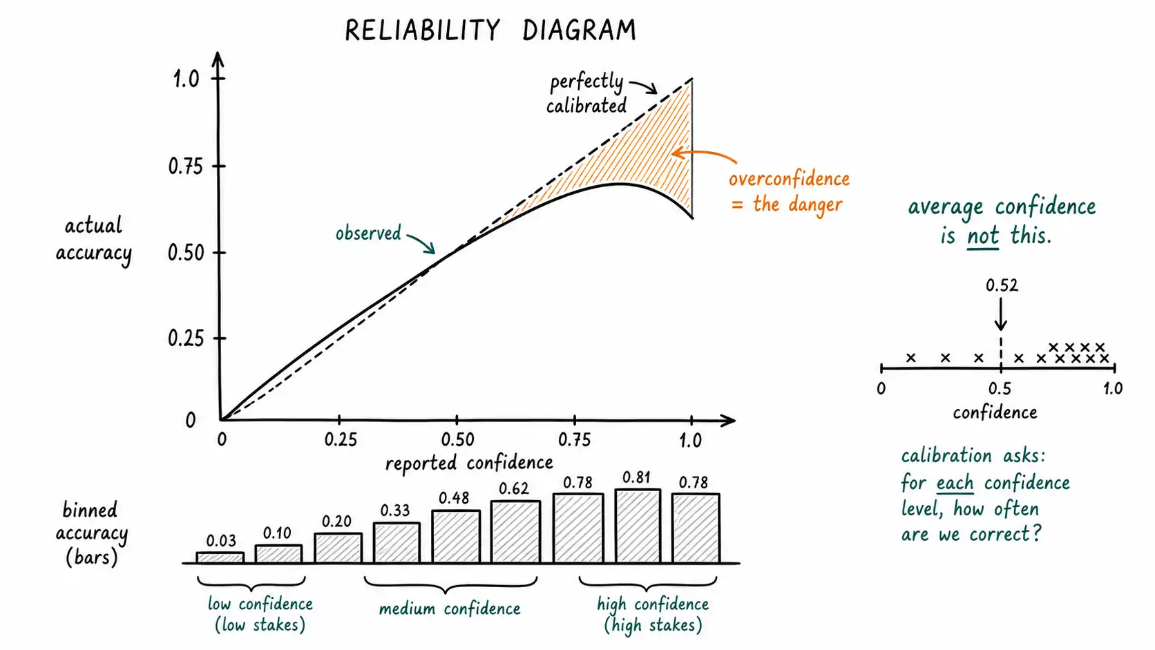
A team once showed me a dashboard with a single number: "model confidence: 0.91 average." They were proud of it. I asked what it meant. It meant the model, on average, reported being 91 percent sure. It said nothing about whether the model was right 91 percent of the time, nothing about whether the cases it was 99 percent sure on were more accurate than the cases it was 60 percent sure on, nothing about whether the confidence was telling the truth. Average confidence is not calibration. It is the model's self-assessment, and we have spent this whole book establishing that the model's self-assessment cannot be taken at face value. This chapter is about measuring calibration properly, which means measuring whether confidence tracks accuracy, and about the specific ways each measurement can mislead you if you are not careful.

The reliability diagram: the picture you should be staring at

The single most useful artifact for calibration is the reliability diagram, sometimes called a calibration plot. It answers the only question that matters: when the system says it is X percent confident, is it actually right X percent of the time?

You build it like this. Take a labeled evaluation set where you know the true answer. For each prediction, record the system's confidence and whether it was correct. Sort predictions into bins by confidence, say ten bins from 0 to 1. For each bin, compute two things: the average confidence the system reported in that bin, and the actual fraction correct in that bin. Plot reported confidence on the x-axis against actual accuracy on the y-axis.

A perfectly calibrated system lies on the diagonal: in the bin where it said 70 percent, it was right 70 percent of the time. The Guo paper that we keep returning to, On Calibration of Modern Neural Networks, uses exactly these diagrams to show that modern networks sit below the diagonal in the high-confidence bins, meaning that when they say 95 percent, they are right less often than 95 percent. They are overconfident, and the diagram shows it as a gap below the line precisely where it hurts most: in the high-confidence region where users have stopped checking.

The reliability diagram is the picture of the enemy. The gap between the curve and the diagonal, especially in the high-confidence bins, is the confident-wrongness problem rendered visually. If you build only one calibration artifact, build this one, and look specifically at the right side of the plot, the high-confidence region, because that is where overconfidence does its damage.

Expected Calibration Error, and the trap inside it

The reliability diagram is a picture; you also want a number, so you can track calibration over time and across model versions. The common one is Expected Calibration Error, ECE: the average gap between confidence and accuracy across the bins, weighted by how many predictions fall in each bin. Lower is better; zero is perfect calibration. Guo and colleagues popularized ECE as the summary statistic for the diagram.

ECE is useful, but it has traps you must know or it will lie to you.

The binning trap. ECE depends on how you bin. Too few bins and you average away real miscalibration; too many and the bins get noisy with too few samples each. Two teams reporting different ECE numbers may just be binning differently. Always report the binning scheme, and prefer looking at the diagram alongside the number rather than trusting the number alone.

The cancellation trap. ECE can hide compensating errors. A system that is overconfident in one region and underconfident in another can post a deceptively low ECE because the errors partially cancel in the average. The diagram shows this; the single number does not. This is the strongest reason to never report ECE without the diagram beside it.

The aggregate trap, which is the most dangerous for product work. Overall ECE can look fine while specific high-stakes slices are badly miscalibrated. Your system might be well calibrated on average and severely overconfident specifically on refund-eligibility questions, the exact slice where errors are expensive. A single global ECE will never surface this. You must compute calibration per slice, per answer type, per source-quality tier, per user segment, because aggregate calibration is cold comfort if the danger-zone slice is the miscalibrated one. This is where the Confidence-Cost Matrix and calibration measurement meet: measure calibration where the matrix says errors are expensive, not just in aggregate.

Proper scoring rules: rewarding honest confidence

There is a deeper tool than ECE, and it matters because of what it incentivizes. A proper scoring rule is a way of scoring probabilistic predictions such that the best possible score is achieved only by reporting your true probability. In other words, a proper scoring rule rewards honesty about confidence and penalizes both overconfidence and underconfidence.

The two canonical proper scoring rules are the Brier score (the mean squared difference between predicted probability and outcome) and the logarithmic score (the negative log of the probability assigned to the true outcome). The foundational treatment is Gneiting and Raftery's Strictly Proper Scoring Rules, Prediction, and Estimation, which is the reference for why these scores have the honesty property and why improper alternatives lead systems to game their reported confidence.

Why does this matter for products and not just for academics? Because the metric you optimize is the behavior you get. If you reward accuracy alone, you incentivize confident guessing, since a confident guess that happens to be right scores the same as a confident correct answer. If you reward a proper scoring rule, you incentivize the system, and the team tuning it, to report confidence honestly, because the only way to optimize the score is to be calibrated. When you build evaluation for a high-stakes AI feature, include a proper scoring rule alongside accuracy. Accuracy tells you how often it is right; the proper scoring rule tells you whether its confidence is honest, and the second is what protects you from confident wrongness.

The log score has a useful property worth highlighting: it punishes confident errors brutally. Being 99 percent confident in a wrong answer earns a near-infinite penalty under the log score. This is exactly the failure mode this book is about, and the log score is the metric that screams loudest about it. If you want a single number that hates confident wrongness, the log score is it.

A worked example you can run by hand

Suppose your support assistant produces these ten predictions on refund-eligibility questions, with the confidence it reported and whether it turned out correct.

Confidence	Correct?
0.95	no
0.95	yes
0.90	yes
0.90	no
0.85	yes
0.80	yes
0.70	yes
0.60	no
0.55	yes
0.50	no

Group the four 0.90+ predictions: average reported confidence about 0.925, actual accuracy 2 of 4 = 0.50. That is a 0.42 gap, severe overconfidence in the high-confidence bin, the exact region where users stopped checking. The average confidence across all ten is 0.77 and the overall accuracy is 0.60, so even the crude "average confidence vs accuracy" comparison shows a 0.17 gap, but it badly understates the problem, because the dangerous overconfidence is concentrated in the high-confidence cases and the aggregate dilutes it. This is the aggregate trap in miniature. The slice that matters, high-confidence refund answers, is far worse calibrated than the global number suggests, and only binning and slicing reveal it.

If this were your real data, the action is clear: the system is overconfident on high-stakes refund answers, so either recalibrate (temperature scaling or similar), raise the abstention threshold so you stop answering in the unreliable high-confidence band, or both. The measurement directly drives the operating-point decision from the abstention chapter.

Calibration is not free and it drifts

Two operational realities that teams discover the hard way.

First, you need labeled data to measure calibration, and getting it for generative, open-ended outputs is genuinely hard. For classification and bounded decisions it is tractable: you have ground truth. For open-ended answers you need a labeling process, human judgment or a trusted automated check, to decide correctness, and that process has its own cost and its own error rate. Budget for it. A calibration program with no labeled data is a wish, not a measurement. Start with the bounded, high-stakes slices where labeling is feasible, the eligibility and routing and extraction decisions, and expand from there.

Second, calibration drifts. The world changes, your data changes, your model changes, your traffic changes. A system calibrated in March can be miscalibrated by September because the distribution of questions shifted or a model update changed the confidence behavior. The Guo result is a warning here too: a model update that improves accuracy can simultaneously worsen calibration. So calibration is not a launch gate you pass once; it is a monitored property with drift detection. Recompute it on a schedule and after every model change, and watch the high-confidence bins for the overconfidence creeping back.

Connecting measurement to the rest of the system

Calibration measurement is not a standalone academic exercise; it feeds every other framework in the book, and that is how you know your measurement program is real rather than decorative.

It sets the thresholds in the answer contract. The confidence bands, high, middle, low, floor, should be set where the reliability diagram says they correspond to real accuracy levels, not picked arbitrarily.

It sets the operating point for abstention. The risk-coverage curve is built from the same labeled data, and the threshold you choose to hit a target error rate comes directly from this measurement.

It validates the Doubt UX Ladder. If your rung-selection policy fires strong doubt signals on cases that turn out to be high-accuracy, your doubt is miscalibrated and you are crying wolf; the measurement tells you so.

It populates the Confidence-Cost Matrix with real numbers. The "apparent confidence" axis can be grounded in measured calibration rather than guessed.

And it is the evidence you bring to governance. When the NIST AI RMF Measure function, which we will treat in the governance discussion, asks how you assess your AI system's trustworthiness, reliability diagrams, sliced ECE, and proper-scoring-rule trends are the concrete answer. Calibration measurement is what makes "we manage AI risk" a checkable claim instead of an assertion.

Practical exercise: the calibration evaluation checklist

Run this on one high-stakes answer type. Treat each item as pass or fail.

1. Do you have a labeled evaluation set for this answer type that resembles production traffic? If not, build it before anything else.
2. Can you extract a confidence number per answer, and is it the same number your interface's expressed confidence is based on? If the interface confidence and the measured confidence are different things, fix that first.
3. Have you built a reliability diagram and looked specifically at the high-confidence bins for overconfidence?
4. Have you computed ECE, reported your binning scheme, and checked for the cancellation and aggregate traps by also computing it per slice?
5. Have you included a proper scoring rule, Brier or log, and looked at whether confident errors are being punished?
6. Have you sliced calibration by the dimensions that matter, answer type, source quality, user segment, so aggregate calibration is not hiding a miscalibrated danger-zone slice?
7. Do you recompute all of the above on a schedule and after every model change, with drift detection?
8. Do the measured bands actually drive the answer contract thresholds and the abstention operating point, or are those still set by guesswork?

A calibration program that passes all eight is the difference between a team that hopes its AI is trustworthy and a team that can prove how trustworthy it is and exactly where it is not. The second team is the one that does not get surprised by a confident wrong answer in production, because they already measured the slice where it was going to happen.

Summary

Average confidence is not calibration; calibration is whether confidence tracks accuracy. The reliability diagram plots reported confidence against actual accuracy and shows overconfidence as a gap below the diagonal in the high-confidence region, exactly where it hurts. ECE summarizes that gap into a number but has three traps: binning sensitivity, error cancellation, and the aggregate trap where global calibration hides a miscalibrated high-stakes slice, so always pair ECE with the diagram and slice it. Proper scoring rules (Brier, log) reward honest confidence and punish confident errors, the log score most brutally, so include one in evaluation to incentivize calibration rather than confident guessing. Calibration needs labeled data, which is hard for open-ended outputs, and it drifts, so it is a monitored property recomputed after every model change. Measurement feeds every other framework: contract thresholds, abstention operating points, ladder validation, the matrix, and governance evidence. Retrieval Quality as a Confidence Signal shows how to extend that measurement upstream - using the retrieval stack itself as a leading indicator before the model even speaks.

Key Takeaways

• Average confidence is the model's self-assessment, not calibration; calibration is whether confidence tracks accuracy, shown by the reliability diagram.
• Look at the high-confidence bins of the reliability diagram; the gap below the diagonal there is the confident-wrongness problem made visible.
• ECE has three traps: binning sensitivity, error cancellation, and the aggregate trap; always pair it with the diagram and compute it per high-stakes slice.
• Proper scoring rules (Brier, log) reward honest confidence; the log score punishes confident errors most severely, making it the metric that hates confident wrongness.
• Calibration needs labeled data and drifts over time and with model updates, so it is a monitored property, not a one-time launch gate.
• Measurement is load-bearing: it sets contract thresholds and abstention operating points, validates the Doubt UX Ladder, and is the concrete evidence for governance.