Scaling Laws in Plain English

The durable AI moat is not model cleverness alone; it is the workflow, data, trust, distribution, and evaluation stack that survives scale.

Most strategy meetings about AI run on vibes. Someone says "the models keep getting better," everyone nods, and then the conversation moves on as if "keep getting better" were a weather report rather than a quantity you could put a number on. It is a quantity you can put a number on. That is the unsettling and useful thing about scaling laws: they took the bitter lesson, which sounds like a philosophy, and turned it into something closer to a forecast. You cannot plan against a philosophy. You can plan against a forecast.

I am not going to derive anything. There is a chapter's worth of math in the source papers and I will link them. What I want is for you to leave this chapter able to do three things: explain to a non-technical board member why models predictably improve, estimate roughly how much a given improvement costs, and recognize when a competitor's "our model is better" claim is a temporary artifact of who spent more compute this quarter rather than a durable advantage.

The one idea: loss falls as a power law in compute, data, and parameters

In January 2020, a team at OpenAI published Scaling Laws for Neural Language Models. The finding, stripped to its core, is this: the loss of a language model, which is a measure of how badly it predicts the next token, falls smoothly and predictably as you increase three things, the number of parameters in the model, the amount of training data, and the amount of compute spent training. The relationship is a power law, which means that on a log-log plot it is a straight line. The paper reports these trends holding across more than seven orders of magnitude. Other architectural details, like exactly how wide or deep the network is, mattered surprisingly little within a broad range.

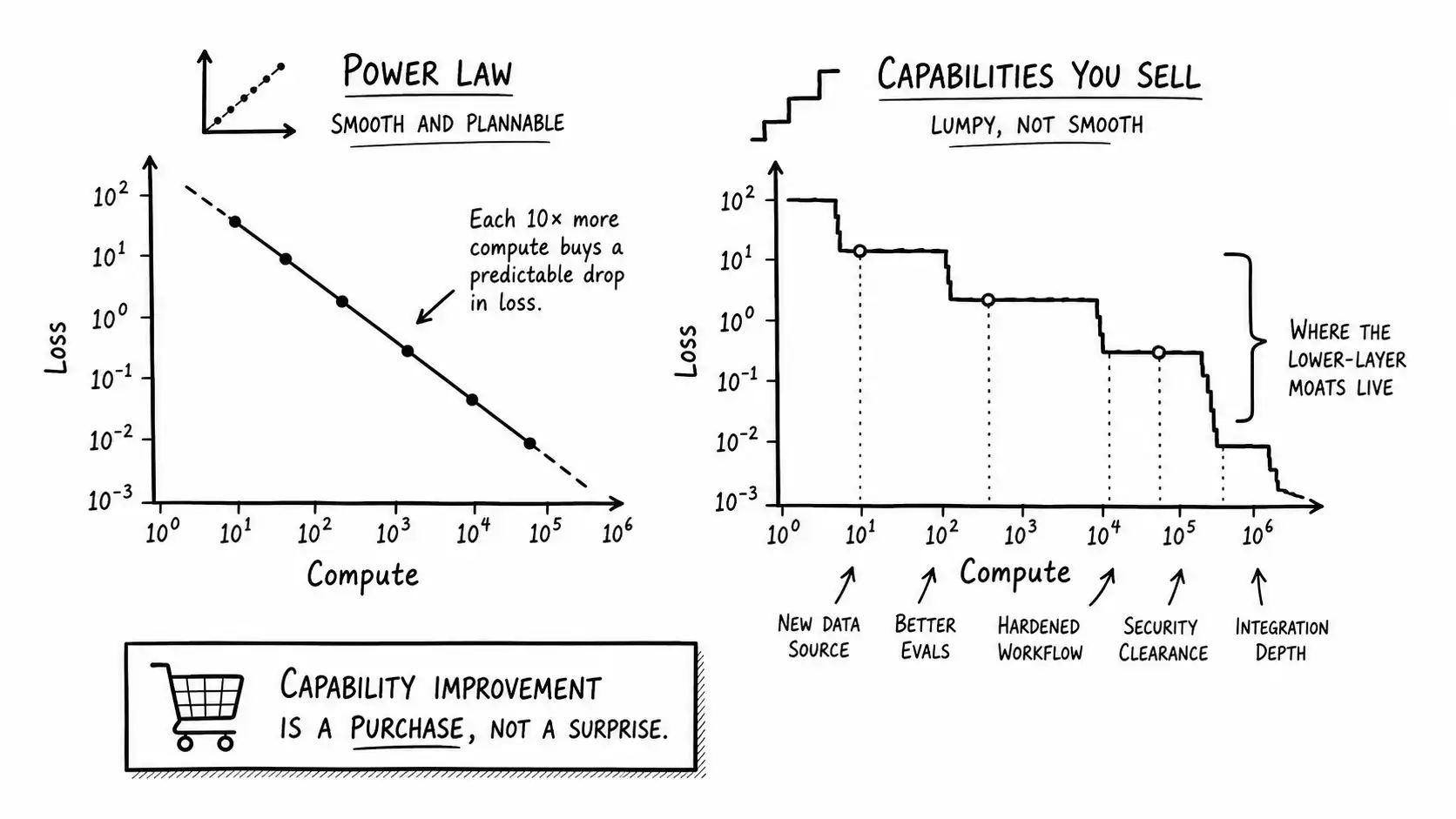
Sit with that for a second, because it is the whole game. A straight line on a log-log plot is the most plannable thing in the world. It means that if you know where you are on the line and you know how much more compute you are about to spend, you can predict roughly how much better the model will be, before you train it. The improvement is not a surprise. It is not luck. It is not a breakthrough you wait for. It is a purchase. You spend compute and you get loss reduction, on a curve you can extrapolate.

This is why "the models keep getting better" is not a vibe. It is the visible surface of a power law that several labs are riding deliberately. They are not hoping the next model is better. They are buying a known amount of better with a known amount of compute.

For the board member: the right mental model is not "the labs are geniuses who keep having breakthroughs." It is "the labs found a curve where money turns into capability at a predictable exchange rate, and they are spending money." That reframing changes how you value a competitor's model lead. A lead bought by spending more compute this quarter is a lead that can be bought back by anyone willing to spend next quarter.

The Chinchilla correction: most early models were the wrong shape

The 2020 paper had a practical implication that turned out to be slightly off, and the correction is worth understanding because it changed the economics.

The early reading of the scaling laws pushed labs toward very large models trained on relatively modest amounts of data. The first wave of giant models, including GPT-3, were built this way: enormous parameter counts, comparatively little training data per parameter. In 2022, a DeepMind team published the work usually called Chinchilla (Hoffmann et al., "Training Compute-Optimal Large Language Models"), which re-examined the question of how to split a fixed compute budget between model size and training data. Their answer: the earlier models were too big and undertrained. For a given compute budget, you should scale parameters and data roughly together, and the compute-optimal ratio they found was on the order of 20 training tokens per parameter. Their demonstration was a model called Chinchilla, 70 billion parameters trained on about 1.4 trillion tokens, which outperformed much larger models trained on less data.

Why does a strategist care about a tokens-per-parameter ratio? Two reasons.

First, it means a smaller model trained correctly can beat a larger model trained wastefully. The advantage of "we have the biggest model" evaporated. The advantage became "we trained the right-sized model on enough good data," which is a more achievable target for more players, which means more competition at the frontier, which means faster commoditization of any given capability level. Chinchilla made the frontier more crowded.

Second, it shifted where the scarce resource sits. If you need roughly 20 tokens per parameter to train compute-optimally, then at large parameter counts you need an enormous amount of high-quality training data. Data quantity and quality became a binding constraint, not just compute. Hold that thought, because it is the bridge to a later chapter on data moats: scaling laws are part of why some data is strategically valuable and most data is not.

Why the curve keeps moving: compute is getting cheaper and bigger fast

A power law is only useful if you know how fast you are moving along it. The answer comes from compute-trend reporting, and the numbers are aggressive.

Epoch AI, which tracks the compute used to train notable models, reports that training compute for frontier models has been growing on the order of 4 to 5 times per year, with the broader trend since 2010 around 4.4 times per year and the language-model frontier specifically closer to 5 times per year, a doubling roughly every six months or so. Three things drive it: more chips running in parallel, longer training runs, and more powerful individual processors. Epoch also notes the cost of these training runs climbing several times per year and the power draw of frontier runs reaching the scale of a medium power plant.

Put the two facts together. Capability improves as a power law in compute, and compute is growing several times per year. That is the engine under "the models keep getting better." It is not slowing on the timescale of your strategic plan, and you should not build a plan that quietly assumes it will. If your plan only works if frontier capability stalls, you do not have a plan, you have a bet against a curve that has held across orders of magnitude.

What scaling laws do not promise, which is the part people forget

Here is where I push back on the hype, because the scaling-law literature is routinely abused to argue more than it shows.

Scaling laws describe the training loss, the model's ability to predict the next token on its training distribution. Lower loss correlates with better performance on many tasks, but the mapping from loss to the specific capability you care about, your extraction accuracy, your tool-use reliability, your refusal behavior on edge cases, is not itself a clean power law. A model can get measurably better at next-token prediction and barely move on your benchmark, because your benchmark depends on something the loss reduction did not happen to improve. The curve is smooth in loss. It is lumpy in the capabilities you actually sell against.

This is the strategist's loophole, and it is real. The lumpiness is exactly where the layers above the model live. A general model getting better at predicting text does not automatically get better at operating inside your customer's permission model, calling your customer's twelve internal systems in the right order, or knowing which of your customer's three conflicting data sources is authoritative. Those are not next-token problems. The smooth curve does not reach them by default.

So the honest summary is: at the model layer, assume the curve. Capability will keep improving on a schedule you do not control, and any advantage that is really a capability gap will close. Above the model layer, the curve does not automatically apply, and that is the only reason this book is more than one sentence long.

A simple way to estimate the cost of a capability gap

Let me make this concrete with a back-of-the-envelope model you can run in a meeting. This is a deliberate simplification, label it as such, but it gets the orders of magnitude right.

Suppose a competitor has a model that is one "capability generation" ahead of the general API you would use. Roughly speaking, in the current regime, a capability generation has tended to cost something like a multiple of compute, call it 5 to 10 times, given the yearly growth rates above. The questions to ask are:

1. How long until the general API reaches the capability your competitor has today? If the frontier moves several times per year, a one-generation lead is on the order of months to a year, not years.
2. What did your competitor spend to open that lead, and can they keep spending to maintain it? A lead funded by a one-time training run is not a lead, it is a depreciating asset.
3. When the gap closes, what does your competitor still have? If the answer is "nothing but the model," they had no moat, only a head start, exactly like the historical cases in the previous chapter.

You do not need precise numbers to use this. The structure forces the right conversation: a model lead has a half-life, the half-life is short and getting shorter, and the only durable question is what survives the gap closing.

A plain-English glossary for the board

Because you will have to explain this to people who will not read the papers, here is the translation layer.

Term	Plain English	Why a strategist cares
Scaling law	Model error falls predictably as you add compute, data, and parameters	Capability improvement is a purchase, not a surprise
Power law	A straight line on a log-log chart	The future point on the line is extrapolatable today
Loss	How badly the model predicts the next token	The thing that improves smoothly, but not the thing you sell
Compute-optimal	The best split of a compute budget between model size and data	Smaller, well-trained models beat bigger wasteful ones
Chinchilla ratio	Roughly 20 training tokens per parameter	Data quantity and quality became a binding constraint
Compute trend	Frontier training compute growing several times per year	The frontier is not stalling on your planning horizon

If a board member remembers only one row, make it the first: capability improvement is a purchase, not a surprise. It defuses the panic that follows a competitor's model announcement, because it reframes the announcement as "they spent money" rather than "they discovered magic."

What to do differently tomorrow

Three concrete moves come straight out of this chapter.

First, stop treating model capability as a roadmap input you control and start treating it as an external curve you forecast. Build your plan to benefit from the curve rising, not to depend on holding a position above it. If a rising frontier helps you, you are aligned with the bitter lesson instead of fighting it.

Second, when a competitor or an internal team claims a model advantage, ask what it cost and what survives it closing. Apply the half-life question. Most claimed model advantages fail this test, and watching one fail it in real time is the fastest way to teach a team the difference between a head start and a moat.

Third, look hard at the gap between the smooth loss curve and the lumpy capabilities you sell. That gap is your strategic territory. The scaling laws tell you where the ground is melting. The places the curve does not automatically reach are where the rest of this book goes to work.

The next chapter changes altitude entirely. Instead of the curve, it looks at what foundation models did to the infrastructure underneath everything you build, because the bitter lesson did not just commoditize capability, it reorganized the entire stack you are standing on, as The Moat Migration Stack makes precise.

Key Takeaways

• Scaling laws turn the bitter lesson into a forecast: model loss falls as a predictable power law in compute, data, and parameters, holding across many orders of magnitude.
• Capability improvement at the model layer is a purchase, not a surprise. Labs buy a known amount of better with a known amount of compute.
• The Chinchilla result showed early giant models were undertrained; the compute-optimal ratio is roughly 20 tokens per parameter, which made the frontier more crowded and made data a binding constraint.
• Frontier training compute has been growing several times per year. Do not build a plan that quietly assumes the curve stalls.
• Scaling laws describe loss, which is smooth, not the specific capabilities you sell, which are lumpy. The gap between smooth loss and lumpy capability is your strategic territory.
• For any claimed model advantage, ask what it cost and what survives the gap closing. A lead funded by a one-time training run is a depreciating asset, not a moat.

Internal map

For the larger argument, keep this chapter connected to The Bitter Lesson, Revisited, the judgment economy, the case for smaller models, and A Field Guide to Evals.