Diversity Is a Measurement, Not a Vibe

Key Takeaways

• Diversity Is a Measurement, Not a Vibe treats synthetic data as a governed artifact, not a free replacement for reality.
• The safe use depends on the cell: training, evaluation, red-team, demo, privacy, or lineage all need different gates.
• Generated data earns its keep only when a real anchor, verifier, and owner survive after generation.

**Working claim: ** "We generated diverse examples" is a claim, and like any claim it is either measured or imaginary. Volume is not coverage; ten thousand examples can occupy the same small region you already had. You cannot know whether generation filled a gap until you measure diversity along the axes that matter, lexical, semantic, label, source, and difficulty, and compare the synthetic distribution against a real target.

The claim that hides a measurement

Open almost any synthetic-data pull request and you will find a sentence like "generated 10,000 diverse examples covering the rare intents." The word "diverse" is doing enormous unearned work. It is a vibe, asserted, not a measurement, demonstrated. And it is usually wrong in a specific direction: a language model sampled repeatedly for the "same" thing produces output that is locally varied, different sentences, but globally concentrated, clustering around the model's preferred way of expressing the concept. You get ten thousand rephrasings of three ideas, not ten thousand ideas.

This matters because the entire justification for generating was coverage. The Chapter 1 team generated to cover rare intents and instead covered one style of rare intent ten thousand times. They had volume and believed they had coverage. The only way to know the difference is to measure it, and the measurement is not exotic. This chapter is the toolkit: five diversity axes, each with a concrete metric, each compared against a real target rather than judged in isolation.

The deep reason this is non-negotiable connects to model collapse. The Curse of Recursion and the Nature collapse work show that the first thing to disappear when you generate from a model is the tail of the distribution, the rare, the weird, the long. A diversity measurement is, in effect, an early-warning system for the tail loss that collapse formalizes over many generations. Measure diversity and you can see, in generation one, the flattening that collapse research shows compounding over many.

Axis 1: lexical diversity

The cheapest axis, and a useful smoke test. Lexical diversity asks how much surface variety exists. The classic measure is the type-token ratio and its length-stable cousins; a more robust signal for generated text is the rate of distinct n-grams.

from collections import Counter

def distinct_n(texts: list[str], n: int = 2) -> float:
 """Fraction of n-grams that are unique. Low = repetitive surface forms."""
 grams = Counter()
 for t in texts:
 toks = t.lower().split()
 for i in range(len(toks) - n + 1):
 grams[tuple(toks[i:i+n])] += 1
 total = sum(grams.values())
 return len(grams) / total if total else 0.0

# Compare synthetic against the REAL anchor, never in isolation:
# distinct_2(real_rare_tickets) -> 0.61
# distinct_2(synth_rare_tickets) -> 0.28 <-- half the surface variety of real

The number alone means nothing. distinct_2 = 0.28 is neither good nor bad until you compare it to the real anchor's 0.61. The comparison is the measurement. Synthetic text with far lower lexical diversity than its real target is reusing phrasing, the generator's house style, and that is the polished-ticket fingerprint showing up as a number you can put in a manifest.

Lexical diversity is a smoke test, not a verdict, because it is fooled in both directions: a generator can produce lexically varied text that is semantically monotonous (different words, same idea), and genuinely diverse real data can be lexically repetitive (terse tickets reuse words). So it screens; it does not decide.

Axis 2: semantic diversity

Semantic diversity is the axis that catches "ten thousand rephrasings of three ideas." Embed the examples, then measure how spread out they are in embedding space and how much they overlap the real distribution. Two complementary metrics:

import numpy as np

def mean_pairwise_distance(embeddings: np.ndarray, sample: int = 2000) -> float:
 """Higher = examples more spread out semantically."""
 idx = np.random.choice(len(embeddings), min(sample, len(embeddings)), replace=False)
 e = embeddings[idx]
 e = e / np.linalg.norm(e, axis=1, keepdims=True)
 sims = e @ e. T
 n = len(e)
 off_diag = (sims.sum() - n) / (n * n - n) # mean cosine sim, excl. self
 return 1.0 - off_diag # convert to a distance

def coverage_of_real(real_emb, synth_emb, radius: float = 0.15) -> float:
 """Fraction of REAL examples that have a synthetic neighbor within radius.
 This is the question that matters: did synthetic data cover the real space?"""
 r = real_emb / np.linalg.norm(real_emb, axis=1, keepdims=True)
 s = synth_emb / np.linalg.norm(synth_emb, axis=1, keepdims=True)
 covered = 0
 for v in r:
 nearest = (s @ v).max() # best cosine sim to any synthetic
 if (1 - nearest) <= radius:
 covered += 1
 return covered / len(r)

coverage_of_real is the single most important diversity number in this chapter, because it answers the actual question: of the real distribution we care about, how much did the synthetic data reach? A team can generate ten thousand examples with high internal spread (mean_pairwise_distance looks great) that nonetheless all sit in one corner of the real space, high internal diversity, low coverage of reality. That is the coverage map from the book prompt made quantitative: the synthetic examples fill some regions and leave others empty, and only coverage_of_real shows you which.

The inverse number matters too. Synthetic examples that land outside any real neighborhood are either valuable novel edge cases or unrealistic fabrications, and you cannot tell which without a human looking. So the embedding map produces a review queue: real regions with no synthetic coverage (the gap you failed to fill) and synthetic regions with no real neighbor (the fabrications you may not want).

Axis 3: label diversity

If you generated to balance classes, measure whether you actually balanced them, and whether the balance is real or assumed. Two distinct checks:

-- Count balance: did we fix the imbalance? (necessary, not sufficient)
SELECT label, COUNT(*) AS n,
 ROUND(100.0 * COUNT(*) / SUM(COUNT(*)) OVER (), 1) AS pct
FROM generated_example
WHERE dataset_id = 'support-intent-synth-v4'
GROUP BY label ORDER BY n DESC;

-- Label-vs-content agreement on the human-reviewed sample:
-- of examples a human reviewed, how often did the prompted label match the text?
SELECT label,
 AVG(CASE WHEN reviewer_label = label THEN 1 ELSE 0 END) AS label_accuracy,
 COUNT(*) AS reviewed
FROM generated_example
WHERE dataset_id = 'support-intent-synth-v4'
 AND human_review_status IN ('approved','rejected')
GROUP BY label;

The first query is the one everyone runs; the second is the one that catches the Chapter 1 failure. A balanced count with low label_accuracy means you have the right number of examples carrying the wrong labels, the assumed-label problem. Balancing the histogram while the labels drift is worse than the original imbalance, because now the model is confidently learning a mislabeled class.

Axis 4: source diversity

Real data comes from many sources, channels, regions, user cohorts, time periods. Synthetic data comes from one generator with, typically, one or a few prompt templates. If your real distribution mixes email, chat, and phone-transcript tickets in some ratio, but your synthetic data is all "generic ticket, " you have collapsed a source dimension that matters. The metric is simply the synthetic source distribution compared against the real one, and the fix is to make source an explicit generation variable: prompt for "an angry chat-channel ticket" and "a forwarded email ticket" as distinct templates, then verify the resulting mix against the real channel mix recorded in your manifest's diversity_strategy.

This is where the Self-Instruct lesson generalizes. Self-Instruct's filtering explicitly rejected new instructions too similar to existing ones, which is a source/semantic diversity gate enforced at generation time rather than measured after. The strongest pipelines do both: force diversity during generation (varied templates, personas, channels) and measure it after (these five axes); the curated-generation results in Textbooks Are All You Need came from exactly this kind of forced, filtered variety rather than raw volume. Forcing without measuring is faith; measuring without forcing is an autopsy.

Axis 5: difficulty diversity

The subtlest axis and the one most often skipped. Generators, left to their defaults, produce easy examples, clear, unambiguous, self-labeling. Real distributions contain a spectrum of difficulty, and the hard cases are usually where the model fails and where you most needed coverage. A difficulty-flat synthetic set teaches a model to handle the easy middle and leaves the hard tail untouched.

You can proxy difficulty several ways: a reference model's confidence (low confidence ≈ hard), human-rated ambiguity, length, or the presence of conflicting signals. Then compare the difficulty histogram of synthetic vs. real:

def difficulty_histogram(texts, model) -> dict:
 """Bucket by reference-model max-class probability; lower prob = harder."""
 buckets = {"easy(>0.9)": 0, "med(0.7-0.9)": 0, "hard(<0.7)": 0}
 for t in texts:
 p = model.predict_proba(t).max()
 if p > 0.9: buckets["easy(>0.9)"] += 1
 elif p > 0.7: buckets["med(0.7-0.9)"] += 1
 else: buckets["hard(<0.7)"] += 1
 return buckets

# real: {'easy': 0.55, 'med': 0.28, 'hard': 0.17}
# synth: {'easy': 0.88, 'med': 0.10, 'hard': 0.02} <-- the generator avoided hard cases

That synthetic histogram is the polished-ticket problem in its purest numeric form: 88% easy versus reality's 55%, and almost no hard cases at all. The generator filled the part of the distribution that was never the problem. Difficulty diversity is also the most direct counter to collapse: the hard tail is precisely what the collapse research shows vanishing first, so a difficulty histogram that under-weights the tail in generation one is the leading edge of the same phenomenon.

A diversity report you attach to the manifest

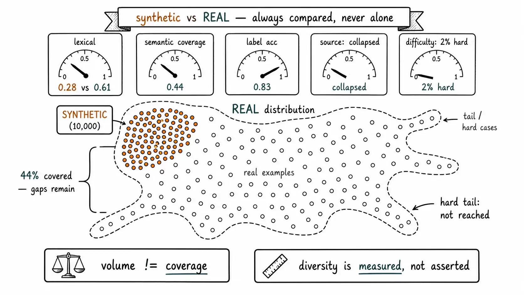
These five axes combine into a single report that travels in the dataset manifest (Chapter 4) and is reviewed before release. The format matters less than the discipline: every number is synthetic compared against real, never synthetic alone.

Axis	Metric	Real anchor	Synthetic	Verdict
Lexical	distinct-2	0.61	0.28	FAIL: half the surface variety
Semantic	coverage_of_real @0.15	-	0.44	FAIL, only 44% of real space reached
Semantic	mean pairwise dist	0.38	0.41	OK internally (misleading alone)
Label	count balance	imbalanced	balanced	PASS
Label	label accuracy (human sample)	n/a	0.83	MARGINAL: 17% mislabeled
Source	channel mix match	email/chat/phone	all generic	FAIL: source collapsed
Difficulty	hard-case fraction	0.17	0.02	FAIL: hard tail absent

This report makes the Chapter 1 disaster legible before training. Internal semantic spread looks fine in isolation, which is exactly why a team reports "it's diverse!", but coverage of real is 44%, the source dimension collapsed to generic, and the hard tail is nearly gone. A team that produced this table would not have shipped; they would have gone back to the generation step with a length-forcing, channel-varying, difficulty-targeting strategy (the v5 diff of Chapter 4) and measured again. The measurement is the difference between a vibe and an engineering control.

Chapter summary

"We generated diverse examples" is a measurement masquerading as a vibe. Language models sampled repeatedly produce locally varied but globally concentrated output, many rephrasings of few ideas, so volume routinely masquerades as coverage. Five axes make diversity an engineering control, each meaningful only when synthetic is compared against a real anchor: lexical (distinct-n surface variety, a smoke test fooled in both directions), semantic (mean pairwise distance for internal spread, and the decisive coverage-of-real metric for how much of the real space was reached), label (count balance plus the often-skipped label-accuracy check that catches assumed labels), source (channel/region/cohort mix, best forced during generation and verified after), and difficulty (a confidence-proxy histogram that exposes the generator's preference for easy, self-labeling examples). A diversity report attached to the manifest renders the Chapter 1 disaster legible before training: internal spread can look fine while coverage is 44%, source has collapsed to generic, and the hard tail, exactly what model-collapse research shows vanishes first, is nearly absent. Measuring diversity in generation one is an early-warning system for the tail loss that collapse formalizes over many generations; forcing diversity without measuring it is faith, and measuring without forcing is an autopsy.