Mixture Ratios, Anchors, and Post-Training Monitoring

Key Takeaways

• Mixture Ratios, Anchors, and Post-Training Monitoring treats synthetic data as a governed artifact, not a free replacement for reality.
• The safe use depends on the cell: training, evaluation, red-team, demo, privacy, or lineage all need different gates.
• Generated data earns its keep only when a real anchor, verifier, and owner survive after generation.

**Working claim: ** The anchor that arrests collapse is not a one-time decision; it is a standing ratio you set per use case and a drift you watch for after the model ships. Synthetic-data failures in production do not announce themselves, the rare case simply stops being handled, so the only defense is monitoring slices you chose before training, against a real-data baseline you protected.

From "anchor exists" to "anchor is maintained"

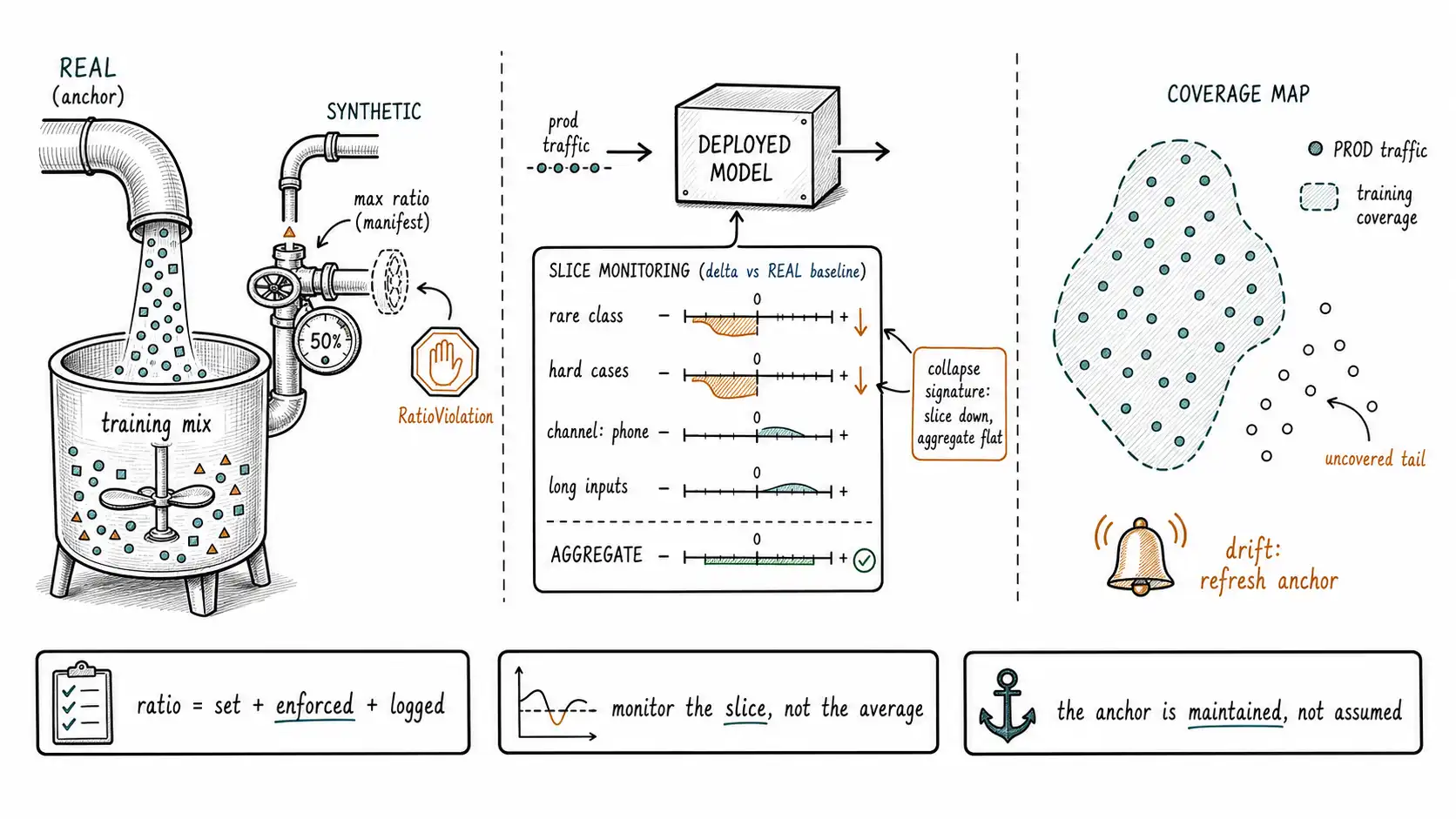
Chapter 10 ended with a result: fresh real data, re-injected, arrests collapse. That is a principle. This chapter turns it into two operational disciplines, because principles do not survive contact with a training pipeline that has a deadline. The first discipline is the mixture ratio: a deliberate, per-use-case cap on how much of a training mix may be synthetic, recorded in the manifest and enforced at build time. The second is post-training monitoring: production slices, chosen before training, that watch for the silent degradation synthetic data causes: degradation that, by its nature, will not show up in your aggregate metrics.

These two disciplines exist because the failure mode is quiet. A model trained on too much synthetic data does not break loudly; it gets slightly worse at the rare cases and slightly better at the common ones, the aggregate metric stays flat or improves, and the failure surfaces weeks later as a pattern of mishandled edge cases that nobody connected to the training mix. The Chapter 1 team's 0.39 production recall was exactly this: invisible in aggregate, fatal in the slice that mattered.

Setting the synthetic ratio

There is no universal safe ratio, because the right cap depends on what the synthetic data is doing and how good your anchor is. But the decision should be explicit and recorded, not an accident of how much data each pipeline happened to produce. Here is a defensible default policy, organized by use case, that a team can adopt and then tune with measurement.

Use case	Suggested max synthetic share	Why	Anchor requirement
Format/paraphrase augmentation	up to ~70%	Low-risk, anchored to real seeds, label preserved	Real seeds for every synthetic variant
Minority-class balancing	~50% of the minority class, not overall	Balances count without flooding; real tail must remain	Real rare examples held aside and included
Edge-case / robustness sets	high within the edge slice, low overall	Edges are deliberately rare; they shouldn't dominate the mix	Real distribution defines the non-edge majority
Instruction/distillation data	varies; filter heavily	The Phi regime works at high synthetic share with heavy filtering	Real or human-aligned teacher; aggressive filtering
Pretraining-scale corpora	low and provenance-tracked	Closest to the collapse regime; uncontrolled accumulation is the risk	Known real fraction; track synthetic provenance
Anything recursive (self-improvement loops)	strict cap + fresh real each round	This is the danger quadrant of Chapter 10	Fresh real data re-injected every iteration

The numbers are starting points, not laws, the Nature work and Curse of Recursion make clear that the safe ratio depends on filtering quality and anchor freshness, and the Phi/Textbooks result shows high synthetic share can be safe when filtering is excellent. The non-negotiable part is not the specific percentage; it is that the ratio is a decision recorded in the manifest (max_synthetic_ratio, Chapter 4) and enforced at build time:

def assemble_training_mix(real, synthetic, manifest) -> list:
 cap = manifest["use_policy"]["max_synthetic_ratio"]
 max_synth = int(len(real) * cap / (1 - cap)) # synth count for target ratio
 if len(synthetic) > max_synth:
 synthetic = downsample_diverse(synthetic, max_synth) # keep diversity (Ch.6)
 mix = real + synthetic
 actual_ratio = len(synthetic) / len(mix)
 if actual_ratio > cap + 1e-6:
 raise RatioViolation(f"synthetic share {actual_ratio:.2%} exceeds cap {cap:.0%}")
 log_mix_composition(manifest["dataset_id"], real=len(real),
 synthetic=len(synthetic), ratio=actual_ratio)
 return mix

Two details matter. The downsampling, when needed, is diversity-preserving (Chapter 6), you drop near-duplicates and over-represented regions first, not random examples, so cutting the synthetic share does not flatten it further. And the actual ratio is logged with the dataset id, so a later regression can be correlated with the mix that produced it, provenance again, applied to the training run rather than the data.

Protecting the real-data baseline

The ratio cap only works if you have real data to anchor against, which means the most precious thing in a synthetic-heavy pipeline is the real data you protected from being diluted, overwritten, or generated-over. Three protections, in order of how often they are violated:

1. **Hold a real anchor out of generation entirely. ** The few real rare examples (the Chapter 1 team's 38 tickets) must never be used as generation seeds in a way that lets the synthetic flood drown them, and must be included in training as the real tail. They are the ground the synthetic data is anchored to.
2. **Hold a real eval out of everything. ** Covered in Chapter 9, restated here because it is the baseline against which you detect collapse. Without a protected real eval, you cannot tell whether a ratio is too high, you have no uncontaminated ruler.
3. **Version the real corpus separately. ** Real and synthetic data should be separately versioned and separately counted (the manifest's by_source_type), so that "we have more data now" can always be decomposed into "more real" versus "more synthetic." A growing dataset that is growing only in its synthetic fraction is drifting toward the collapse regime even if the total looks healthy.

The NIST AI RMF framing of this is data lineage and the ability to characterize your data assets; the operational version is simply never losing track of your real-to-synthetic balance, which the contamination survey repeatedly shows is exactly what teams do lose track of as synthetic data accumulates.

Monitoring slices you chose before training

Aggregate accuracy is where collapse hides. The defense is to define, before training, the slices where synthetic data is most likely to have flattened the distribution, and to monitor those slices in production against the protected real baseline. The slices are predictable from the diversity analysis of Chapter 6: the rare classes, the hard-difficulty bucket, the under-covered source channels, the long tail of input length.

-- Post-deployment slice monitoring. Run on REAL production traffic with
-- ground truth backfilled from human review or downstream signals.
SELECT slice,
 COUNT(*) AS n,
 AVG(CASE WHEN pred = truth THEN 1 ELSE 0 END) AS accuracy,
 AVG(CASE WHEN pred = truth THEN 1 ELSE 0 END)
  - baseline_accuracy AS delta_vs_baseline
FROM prod_predictions p
JOIN slice_definitions s ON p.input_id = s.input_id
JOIN real_baseline b ON s.slice = b.slice -- baseline from PROTECTED real eval
WHERE p.served_at > now() - interval '7 days'
GROUP BY slice, baseline_accuracy
ORDER BY delta_vs_baseline ASC; -- worst-degraded slices first

-- A negative delta on a rare/hard slice while aggregate is flat
-- == the collapse signature: synthetic flattened the tail.

The ORDER BY delta_vs_baseline ASC puts the failing slices first, and the comment names the signature you are hunting: a slice, almost always a rare or hard one, degrading against the real baseline while the aggregate metric stays flat or improves. That divergence between slice and aggregate is the production fingerprint of too much synthetic data, and it is invisible to anyone watching only the top-line number. The Chapter 1 team had no slice monitoring, so the rare-intent collapse was invisible until it became an incident.

A drift detector for the synthetic fingerprint

Beyond accuracy slices, you can monitor the distribution of production inputs against what the model was trained on, watching for the gap between the synthetic-heavy training distribution and the real production distribution. The realism classifier of Chapter 7 reappears here as a drift monitor:

def production_drift(train_emb, prod_emb_window) -> dict:
 """How far is live traffic from the (synthetic-heavy) training distribution?"""
 coverage = coverage_of_real(prod_emb_window, train_emb, radius=0.15) # Ch.6
 # coverage = fraction of PROD inputs that have a near training neighbor.
 # Low coverage = production is in a region training (esp. synthetic) under-covered.
 return {
 "prod_covered_by_train": coverage,
 "alarm": coverage < 0.80, # tune per domain
 "interpretation": "low = synthetic training missed real production regions",}

This flips Chapter 6's coverage metric around: there we asked whether synthetic data covered the real space; here we ask whether the training data (synthetic-heavy) covers the live production space. Low coverage means production traffic is landing in regions the training distribution under-represented, the tail the synthetic data flattened, and it is an early warning that precedes the accuracy degradation, because you see the inputs arriving in uncovered regions before you see the model fail on them.

The standing policy

Monitoring is only useful if someone acts on it, so the disciplines combine into a standing policy with thresholds and owners, in the spirit of the NIST AI RMF "manage" function. The policy is short:

• **Ratio: ** Every training run records its real/synthetic ratio and the manifest cap it respected. A run that needs to exceed the cap requires explicit sign-off, not a silent override.
• **Baseline: ** A protected real eval runs on every candidate model; a synthetic-only eval may supplement but never replace it (Chapter 9).
• **Slices: ** Rare, hard, and under-covered slices are monitored in production weekly against the real baseline; a slice degrading while aggregate is flat triggers investigation of the training mix.
• **Drift: ** Production-vs-training coverage is monitored; a drop below threshold triggers a refresh of the real anchor and re-evaluation of the ratio.
• **Retirement: ** When the real distribution shifts enough that the synthetic data no longer reflects it (the manifest's expires_at, Chapter 4), the dataset is regenerated or retired, not silently reused.

None of this is exotic, and all of it is the operational form of "the anchor is maintained, not assumed." The Chapter 1 failure was not a generation mistake at heart; it was the absence of every item on this list. The team set no ratio, protected no baseline, monitored no slice, watched no drift, and retired no dataset, so when the synthetic data flattened the rare-intent tail, nothing in the system was positioned to notice.

Chapter summary

The anchor that arrests collapse must be maintained, not assumed, through two disciplines. First, a synthetic mixture ratio set per use case (format augmentation tolerates high shares, minority balancing caps at the class level, recursive loops require strict caps plus fresh real data each round), recorded in the manifest and enforced at build time with diversity-preserving downsampling and a logged actual ratio, the specific percentage is tunable but the recorded, enforced decision is not. Second, the real-data baseline must be protected: a real anchor held out of generation and included as the real tail, a real eval held out of everything, and the real corpus versioned and counted separately so "more data" can always be split into more-real versus more-synthetic. The failure mode is quiet, synthetic data flattens the tail while aggregate metrics stay flat, so the defense is monitoring slices chosen before training (rare classes, hard cases, under-covered channels, long inputs) against the protected real baseline, hunting the collapse signature of a slice degrading while the aggregate holds. A production-versus-training coverage monitor flips Chapter 6's metric to catch live traffic landing in regions the synthetic-heavy training under-covered, an early warning before accuracy drops. These combine into a standing policy, ratio sign-off, protected baseline, weekly slice monitoring, drift alarms, dataset retirement, whose total absence was the true Chapter 1 failure.