Difficulty From History: Slices, Embeddings, and Learned Routers

Key Takeaways

• Difficulty From History: Slices, Embeddings, and Learned Routers is a chapter about model routing and inference control planes, not a generic AI adoption note.
• The operating rule is to send each request to the cheapest path that still meets quality, latency, residency, and risk requirements.
• The failure mode to watch is polished output without evidence, owner, cost line, or rollback path.
• The useful next step is an artifact a future teammate can replay without folklore.

Model routing works when each request goes to the cheapest path that still meets quality, latency, residency, and risk requirements.

Working claim: The strongest difficulty signal is not in the request; it is in your logs."Requests like this one", same task type, same domain, same shape, have a measured track record of how often each model got them right. A router that consults that history routes on evidence; a router that guesses from the prompt alone routes on intuition. The path from a heuristic router to a learned one runs through the decision log, and you cannot skip it.

The signal that beats all the others

Chapters 4 through 6 ranked difficulty signals and kept arriving at the same conclusion: the cheap, immediate signals (length, verbalized confidence) are weak, and the strong signals require infrastructure. This chapter is about the strongest signal of all, and it is not in the request, it is in what happened the last ten thousand times you saw a request like this one.

The idea is simple and the implications are large. Group your historical requests into slices, equivalence classes of "requests like this", and for each slice, measure what each model actually achieved: accuracy, escalation rate, cost, latency. Then a new request's difficulty is not predicted from its words; it is looked up from the track record of its slice."Billing disputes with a refund mentioned" might have a measured cheap-model accuracy of 62%; "shipping status lookups" might be 99%. Those numbers are not guesses. They are observations, and observations beat predictions.

This is why the decision log from Chapter 1 was not optional plumbing. A router that does not log its decisions and their outcomes can never learn from history, because it has no history, it is condemned to re-guess from the prompt forever. The decision log plus eventual quality labels (Chapter 14) is the training data for everything in this chapter. Build the log first; the learned router is downstream of it.

What a slice is

A slice is a set of requests you are willing to treat as interchangeable for routing purposes: similar enough that their model performance is similar. The art is choosing the slicing dimensions coarse enough to have data in each slice but fine enough that the slices are actually homogeneous in difficulty. Common dimensions:

• Task type / intent (the strongest single dimension): summarization, extraction, code-gen, arithmetic, multi-doc QA, classification.
• Domain: billing, shipping, legal, medical, technical-support.
• Structural features: needs-retrieval, needs-tools, multi-turn, single-shot.
• Tenant or product surface: different customers send different difficulty mixes.

The slice key is just a tuple of these. The trick is to start coarse (task type alone) and refine only where the data shows a slice is heterogeneous, where the cheap model's accuracy within the slice has high variance, indicating you have lumped easy and hard requests together. Refining a heterogeneous slice is how you discover, for instance, that "billing" is fine for the cheap model except when a dispute and a refund are both mentioned.

-- The core slice-performance query. This IS the router's knowledge base.
-- Run it nightly; the routing policy reads from a materialized version.

SELECT
 task_type,
 domain,
 model,
 count(*) AS n,
 avg(case when quality_label = 'pass' then 1.0 else 0.0 end) AS accuracy,
 avg(case when escalated then 1.0 else 0.0 end) AS escalation_rate,
 avg(cost_usd) AS mean_cost,
 percentile_cont(0.95) within group (order by latency_ms) AS p95_latency
FROM routing_outcomes
WHERE ts > now() - interval '30 days'
 AND quality_label IS NOT NULL -- only labeled outcomes (Ch. 14)
GROUP BY task_type, domain, model
HAVING count(*) >= 50 -- ignore slices too small to trust
ORDER BY task_type, domain, accuracy DESC;

The HAVING count(*) >= 50 matters: a slice with five observations is a rumor, not a track record, and routing on it is overfitting to noise. New or rare slices fall back to a conservative default (a higher tier or a cascade) until they accumulate enough data to trust. This is the cold-start problem, and the safe answer to cold-start is route up, treat unknown slices as harder than you hope, the same conservatism risk demanded in Chapter 5.

From slice table to routing decision

With a slice-performance table, routing becomes an expected-value calculation against the slice's measured numbers. For a new request, look up its slice, and for each eligible model (eligibility already filtered by risk and length, per Chapters 4-5), the router has measured accuracy, cost, and latency. The cheapest model whose measured accuracy on this slice clears the slice's quality bar is the answer.

# Routing as a lookup against measured slice performance.
# No guessing from the prompt - this is evidence-based routing.

def route_from_history(request, slice_table, fleet):
 risk = assess_risk(request) # Ch. 5: floor first
 eligible = risk_eligible(fleet, risk)
 slice_key = (request.task_type, request.domain)
 bar = quality_bar_for(risk) # Ch. 5: bar depends on risk

 perf = slice_table.get(slice_key)
 if perf is None or perf.n < 50: # cold start: route up
 return cheapest(eligible, min_tier="mid-hosted")

 # Cheapest eligible model whose MEASURED accuracy clears the bar.
 candidates = [
 m for m in eligible
 if perf.accuracy.get(m, 0.0) >= bar
 ]
 if not candidates:
 return strongest(eligible) # nobody clears it -> top tier
 return min(candidates, key=lambda m: perf.mean_cost[m]) # cheapest that works

This function embodies the book's subtitle precisely: cheapest model whose measured accuracy on this slice clears the bar. It is not clever. Its intelligence is entirely in the data behind slice_table, which is why the logging discipline is the real engineering and the routing function is almost trivial once the data exists.

Embeddings: slices without hand-drawn boundaries

Hand-defined slices have a limit: you can only slice on dimensions you thought of. Some difficulty structure is semantic and doesn't map cleanly to task-type/domain tuples, two requests in the same nominal task type can be very different in difficulty for reasons that live in their meaning. Embeddings let you slice on semantics instead of hand-labeled categories.

The technique: embed each request, and find its nearest neighbors among historical requests whose outcomes you know. The new request's expected difficulty is the model performance on its semantic neighborhood. This is a k-nearest-neighbors router over an embedding space, and it captures difficulty structure no hand-drawn slice can, because the "slice" is defined by semantic proximity, dynamically, per request.

# Embedding-based difficulty: route by the outcomes of semantically similar past requests.

def difficulty_from_neighbors(request, index, k=20):
 vec = embed(request.prompt)
 neighbors = index.search(vec, k=k) # k nearest past requests (with outcomes)
 if not neighbors:
 return None # cold start
 # Cheap model's measured accuracy on the semantic neighborhood:
 cheap_acc = mean(n.was_cheap_model_correct for n in neighbors)
 # Distance-weight so closer neighbors count more (optional refinement).
 return 1.0 - cheap_acc # higher = harder

A caution that connects to the wider series: embedding-based routing is only as good as the embedding's fit to difficulty, and general-purpose embeddings are optimized for semantic similarity, not difficulty similarity. Two requests can be semantically close and differ sharply in difficulty (a simple and a trick version of the same question). Embedding routers work well as a signal among several and poorly as a sole oracle; validate them on held-out outcomes before trusting them, the same evaluation discipline the OpenAI evals guide prescribes for any predictive component.

Learned routers: predicting the winner directly

The most sophisticated approach skips difficulty as an intermediate and predicts the routing decision directly: given a request, which model will produce the better answer? This is what RouteLLM does. It trains a router on human-preference data, pairs where humans judged the strong model's answer better or not-better than the weak model's, to learn, before generation, whether a given query needs the strong model. RouteLLM reports cutting cost "by over 2 times in certain cases, without compromising the quality of responses, " and, notably, that its routers exhibit "significant transfer learning capabilities, " holding up even when the underlying strong and weak models are swapped at test time, meaning the router learned something about query difficulty general enough to survive a model change.

The training-data lesson is the deepest one in the chapter: where do the preference labels come from? Three sources, in increasing cost and quality:

1. Free signals from the cascade itself. Every time your cascade escalates, you get a labeled example: this request, the cheap model's answer, whether the verifier accepted it. Over time the cascade generates its own training data for a predictor that can skip the cheap attempt next time: turning a look-and-climb pattern into a predict-and-commit one for slices it has learned. This is the virtuous loop: cascades produce labels, labels train predictors, predictors reduce cascading cost.
2. Cheap automated graders. Where you have a verifier (tests pass, schema validates), every request is auto-labeled, and you can train a winner-predictor without humans.
3. Human preference labels. The gold standard RouteLLM uses, expensive but most reliable, especially for subjective tasks where no automated verifier exists.

# The virtuous loop: the cascade's own escalation outcomes train a predictor
# that learns to SKIP the cheap attempt on slices where it reliably loses.

def harvest_training_examples(routing_outcomes):
 examples = []
 for o in routing_outcomes:
 if o.lane == "cascade":
 # Label: did the cheap model's answer survive the verifier?
 label = "cheap_sufficient" if not o.escalated else "needed_strong"
 examples.append((features(o.request), label))
 return examples

# Periodically retrain; the predictor lets the router commit instead of cascade
# on confidently-easy and confidently-hard slices (Ch. 3's combined architecture).
winner_predictor.fit(harvest_training_examples(last_30_days))

The maturity ladder

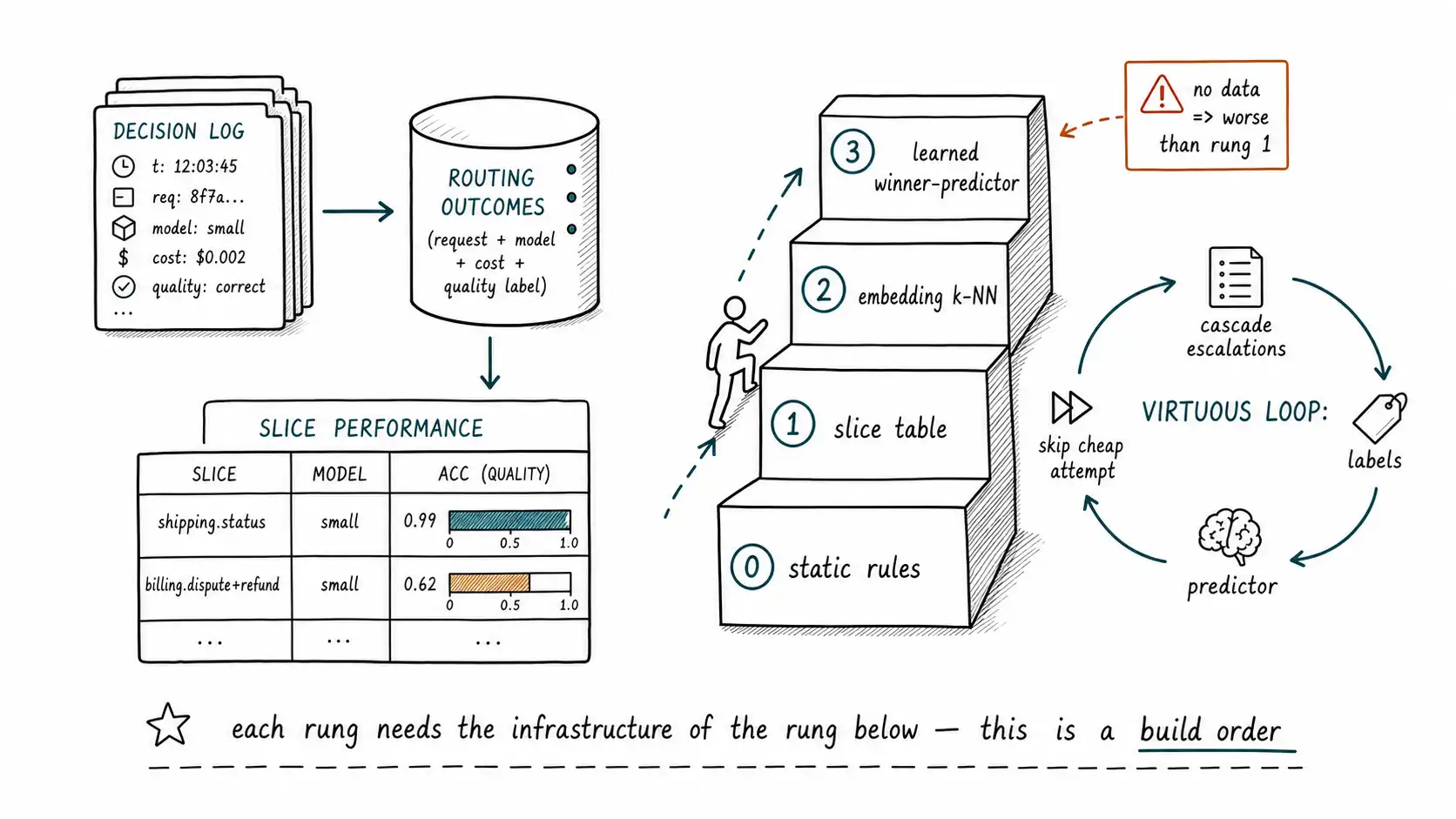
These approaches are not competitors; they are a maturity ladder, and most teams should climb it in order rather than jumping to the top.

Rung	Signal	Needs	Good for
0	Static rules (task type)	Nothing	Day one; obvious task splits
1	Hand-defined slice table	Logged outcomes + labels	Most production systems; interpretable
2	Embedding k-NN difficulty	Embedded log + outcomes	Capturing semantic difficulty structure
3	Learned winner-predictor	Labeled preference/verifier data	Skipping cascades; subjective tasks

The trap is skipping straight to rung 3 because it sounds best. A learned router with no data is worse than a hand-written slice table, and a slice table with no logged outcomes is impossible. Each rung requires the infrastructure of the rung below it, outcomes logged, slices defined, embeddings indexed, so the ladder is also a build order. The reward for climbing it is that the router stops guessing from the prompt and starts routing on what its own traffic taught it, which is the difference between a router that ages into wisdom and one that re-makes the same mistakes forever. FrugalGPT and SelfCheckGPT sit at different rungs: FrugalGPT's learned scorer is rung-3 thinking about stopping, SelfCheckGPT's consistency check is a rung-2 behavioral signal, and a mature router borrows from both.

Chapter summary

The strongest difficulty signal is not in the request but in the logs: group historical requests into slices of "requests like this, " measure what each model actually achieved on each slice, and look up a new request's expected difficulty from its slice's track record, observations beat predictions, which is why the Chapter 1 decision log was never optional plumbing but the training data for everything here. Slices are tuples of task type, domain, and structural features; start coarse and refine only where a slice's cheap-model accuracy shows high variance (the tell that you lumped easy and hard together), and never route on a slice with too few observations, cold-start means route up. Routing then becomes a lookup: the cheapest risk-eligible model whose measured accuracy on this slice clears the risk-set quality bar, which is the book's subtitle made literal. Embeddings extend slicing to semantic neighborhoods via a k-NN difficulty estimate, capturing structure hand-drawn slices miss, but general embeddings track semantic, not difficulty, similarity, so validate them on held-out outcomes and use them as one signal among several. The most sophisticated approach, RouteLLM, trains a winner-predictor directly on preference data and even transfers across swapped models, and its training labels come from a virtuous loop: the cascade's own escalation outcomes label which requests needed the strong model, letting the router learn to skip the cheap attempt on slices where it reliably loses. These form a maturity ladder (static rules → slice table → embedding k-NN → learned predictor) that is also a build order, because each rung requires the infrastructure of the one below, and jumping to a learned router with no data is worse than a hand-written slice table.

Internal map

For the larger argument, keep this chapter connected to Model Routing, The Economics of Inference, the smaller-model margin argument, and A Field Guide to Evals.